Introduction

We propose four algorithms for computing the inverse optical flow between two images. We assume that the forward optical flow has already been obtained and we need to estimate the flow in the backward direction. The forward and backward flows can be related through a warping formula, which allows us to propose very efficient algorithms. These are presented in increasing order of complexity. The proposed methods provide high accuracy with low memory requirements and low running times. In general, the processing reduces to one or two image passes. Typically, when objects move in a sequence, some regions may appear or disappear. Finding the inverse flows in these situations is difficult and, in some cases, it is not possible to obtain a correct solution. Our algorithms deal with occlusions very easy and reliably. On the other hand, disocclusions have to be overcome as a post-processing step. We propose three approaches for filling disocclusions. In the experimental results, we use standard synthetic sequences to study the performance of the proposed methods, and show that they yield very accurate solutions. We also analyze the performance of the filling strategies.

In this page you can find the codes for the four implementations of our algorithms.

Full text: Sánchez Pérez, J, Salgado de la Nuez, A.J. & Monzón López, N . (2013) Computing Inverse Optical Flow.CTIM Technical Report.(3).Universidad de Las Palmas de Gran Canaria.

Download source code

InverseFlowCode.zip The software is released under the BSD license

You can compile it executing make on the console. Execute file is a program for testing the method using Grove2 sequence.

Notation and General Framework

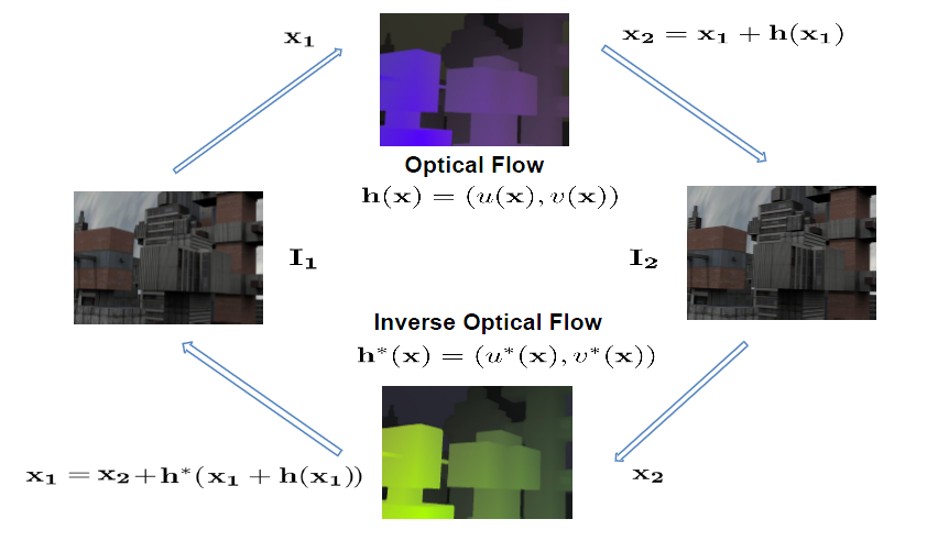
Let I₁(x) and I₂(x) be two color images in a sequence, with x = (x, y), and h(x) = (u(x), v(x)) the vector field that establishes the correspondences between the pixels of the images. h(x) is said to be dense if it is a mapping of every pixel in the first image to the pixels in the second image. We define the backward flow, h^*(x) = (u^*(x), v^*(x)), as the inverse of h(x). h^*(x) puts in correspondence the pixels in the second image with the pixels in the first image. The forward and backward flows can be related as:



This relation can be intuitively derived from the graphic depicted in Fig. 1. The corresponding positions are given by the warping function, x → x + h(x).

Fig. 1. Relation between the forward, h(x), and backward, h*(x), optical flows.

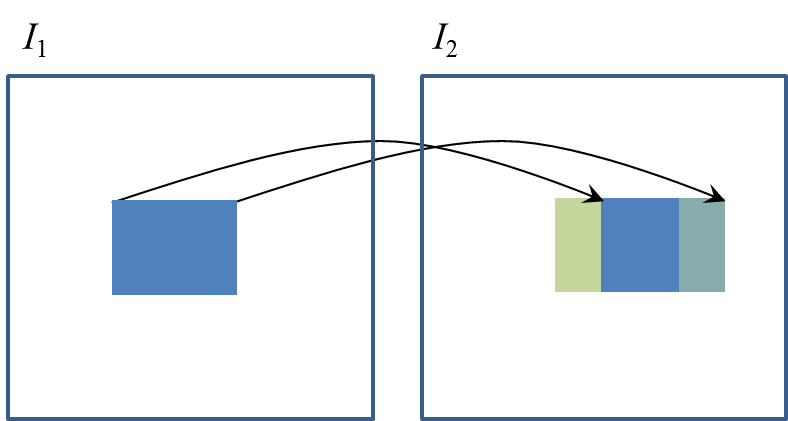
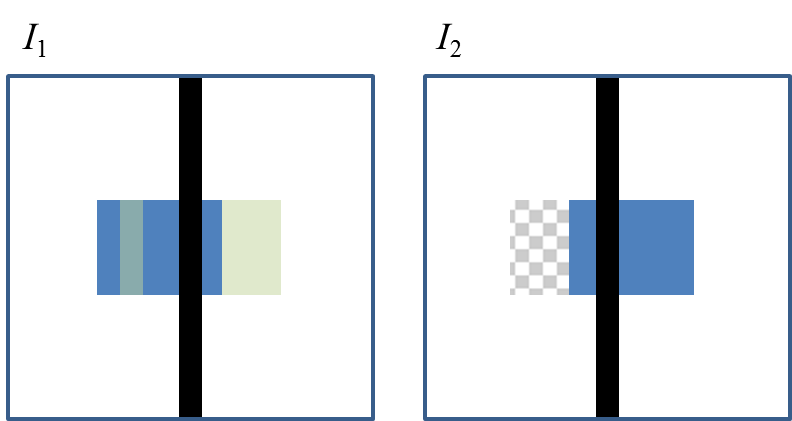
Typically, h(x) is not bijective and it is not possible to estimate h^*(x) in the whole domain. This is true, for instance, in occluded and disoccluded regions: occlusions occur when several correspondences arrive to the same position in the second image; disocclusions occur when an object appears and there is no correspondence in the first image. In this sense, we also find two possible situations: occlusions may appear when moving objects occlude other background objects, like depicted in Fig. 2; on the other hand, occlusions may also occur when objects displace behind other objects, like in Fig. 3. The former situation is typical in fronto-parallel stereoscopic sequences, so we will refer this situation as the stereoscopic occlusion.

Fig. 2. Stereoscopic Occlusion: when the blue square moves horizontally, it creates a disocclusion and occlusion before and after the square, respectively.

Fig. 3. Street-lamp Occlusion: the blue square moves behind the static central bar. Occlusions appear in front of the square and also inside the square, induced by the static bar.

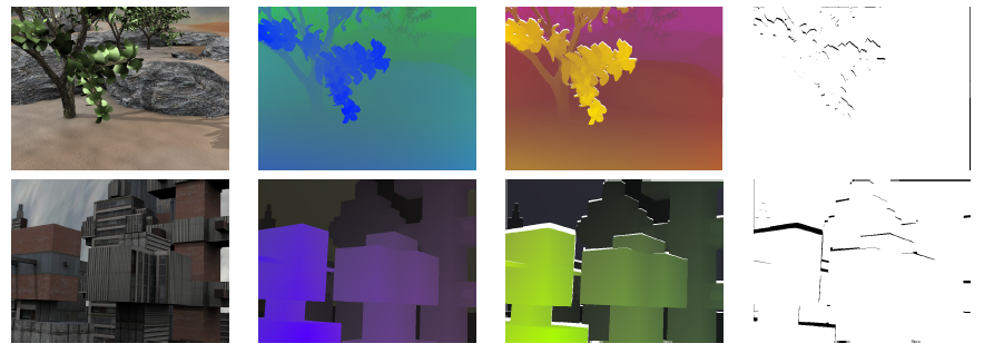
Fig. 4 shows two examples of inverse optical flows. In this case, we have used two sequences from the Middlebury benchmark database. The forward optical flows are known (second column) and the inverse flows are calculated using one of our algorithms (third column). We also show the disocclusion maps in the fourth column. The motion fields are shown using the color scheme depicted in Fig. 5.

Fig. 4. Two examples using sequences from the Middlebury benchmark database: the first column shows the Grove2 and Urban3 sequences, respectively; the second depicts the forward optical flows; the third, the inverse optical flows; and the last one, the corresponding disocclusions.

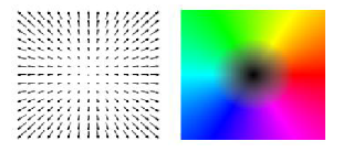
Fig. 5. Color scheme used to represented the optical flows. The colors represent the orientation and magnitude of the flow field.

Examples

This subsection shows several tests with the sequences of the Middlebury benchmark database and Yosemite with clouds using our algorithms. Algorithms 1 and 2 are a nearest neighbor algorithms that use a single value from the forward flow while algorithms 3 and 4 are an interpolation algorithms that compute an average between the values that get close to a position. These are explained in subsections 4.1 and 4.2 of the original CTIM Technical Report, respectively. These categories are further divided in flow- and image-based strategies. The flow-based strategy uses the information of the forward optical flow, whereas the image-based strategy also uses the information of the image intensities.
Figure 6 show the results for Algorithm 1 .

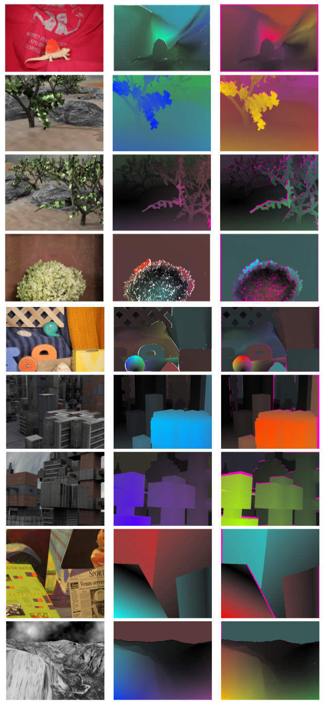
Fig. 6. Middlebury test sequences. First column, the source image; second, the ground truth optical flow; third, the inverse optical flow using Algorithm 1, with disocclusions in pink.

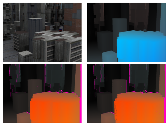
Fig. 7 compares the solution of a flow-based algorithm (Algorithm 1) with respect to an image-based algorithm (Algorithm 2).

Fig. 7. Flow-based versus image-based algorithms. Comparison between Algorithms 1 and 2.

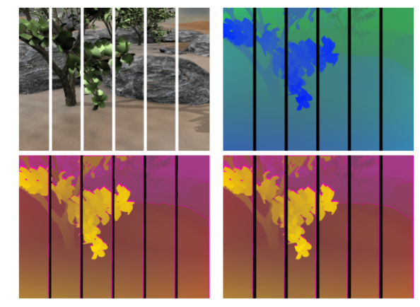
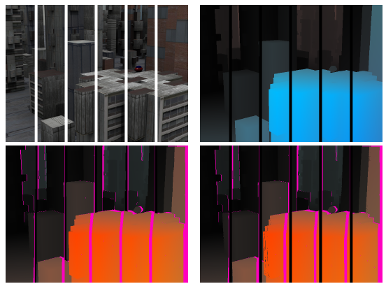
Next, we study the performance of the algorithms with respect to the street-lamp occlusion. We modify two Middlebury sequences, Grove2 and Urban2, adding five static bars in front of the scene. This easily simulates the effect of the objects moving behind a fence. In Fig. 8 we show the results for Grove2 while fig. 9 shows the results for the Urban2 sequence with bars.

Fig. 8. Street-lamp occlusion for Grove2. First row, the source image and the ground truth. Second row, the backward flows for Algorithms 1 and 2.

Fig. 9. Street-lamp occlusion for Urban2. First row, the source image and the ground truth. Second row, the backward flows for Algorithms 1 and 2.

References

1. Javier Sánchez, Agustín Salgado, and Nelson Monzón. Computing inverse optical flow. Pattern Recognition Letters Volume 52, 15 January 2015, Pages 32–39
2. Javier Sánchez, Agustín Salgado, and Nelson Monzón. Direct estimation of the backward flow. In International Conference on Computer Vision Theory and Applications (VISAPP), pages 268–274. Institute for Systems and Technologies of Information, Control and Communication, 2013.
3. Javier Sánchez, Agustín Salgado, and Nelson Monzón. An efficient algorithm for estimating the inverse optical flow. In 6th Iberian Conference on Pattern Recognition and Image Analysis (IbPRIA), pages 390–397. Springer-Verlag, 2013.
4. Javier Sánchez, Agustín Salgado, and Nelson Monzón. Optical flow estimation with consistent spatio-temporal coherence models. In International Conference on Computer Vision Theory and Applications (VISAPP), pages 366–370. Institute for Systems and Technologies of Information, Control and Communication, 2013.

Acknowledgements

This work has been partially supported by the Spanish Ministry of Science and Innovation through the research project TIN2011-25488 and the grant ULPGC011-006.