Introduction
The accuracy and performance of current variational optical flow methods have considerably increased during the last years. The complexity of these techniques is high and enough care has to be taken for the implementation. The aim of this work is to present a comprehensible implementation of recent variational optical flow meth- ods. We start with an energy model that relies on brightness and gradient constancy terms and a flow-based smoothness term. We minimize this energy model and derive an efficient implicit numerical scheme. In the experimental results, we evaluate the accuracy and performance of this implementation with synthetic images. We show that it is a competitive solution with respect to the most accurate methods. In order to increase the performance, we use a simple strategy to parallelize the execution on multi-core processors.Download full text
[1] Sánchez Pérez, J, Monzón López, N & Salgado de la Nuez, A.J.. (2012) Parallel Implementation of a Robust Optical Flow Technique.CTIM Technical Report.(1).Universidad de Las Palmas de Gran Canaria.Download source code
In this page you can find the code for the implementation of a robust variational optical flow method. These are based on energy functionals that include the brightness and gradient constancy assumptions and a flow driven smoothness regularization. These methods replace the traditional quadratic penalty function by a continuous L1 norm, which makes them more robust to noise and outliers. We use the OpenMP library for the parallelization of the algorithms. It is a simple parallelization that does not modify the original code. The code is developed in standard C++ and it has been compiled in Windows and Linux, using the GNU gcc compiler.robust_optic_flow.zip The software is released under the BSD license
You can compile it executing make on the console
Energy model
Let h(x) = (u(x), v(x))T : R2 → R2 , be a vectorial function representing the optical flow field in the continuous domain Ω. For every position x = (x, y)RT , the optical flow depicts a directional vector of the apparent displacement at a given position. The optical flow is an ill-posed problem in the sense that it is not possible to calculate it only from the data. It is necessary to impose a regularity constraint that defines a preferred heuristic solution. In our variational formulation, a general energy model contains a set of constancy and smoothness assumptions that enables us to compute the optical flow by applying optimization techniques. Our energy model can be written as follows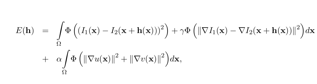
where
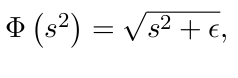 with ε = 0.0001.
The first term, which corresponds to the brightness constancy assumption, attracts pixels with the same intensity in both images. It fails in the presence of noise or changes in illumination. The second term, corresponding to the gradient constancy assumption, compares the structure of the objects in both images: it is invariant to constant changes in illumination, but fails under the presence of noise or in the case of non-translational displacements. Finally, the smoothness term is in charge of creating a continuous and dense solution.
Examples
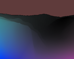
This subsection shows several tests with the sequences in the Middlebury benchmark database and Yosemite with clouds. We have used the color scheme show in Fig 1 to represent the orientation and the magnitude of the flow field in everypoint of the images.

|
| Fig. 1. Color scheme |
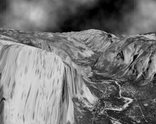
Yosemite Sequence
We have used our method with the parameters shown in Table 1. The results can be seen in Fig 2.| Frame 6 | Ground truth | Best parameters |
|---|---|---|
 |
 |
 |
| Fig. 2. Yosemite with clouds | ||
| α | γ | η | Inner Iter | Outer Iter | EPE | AAE |
|---|---|---|---|---|---|---|
| 250 | 37 | 0.5 | 25 | 100 | 0.098 | 2.190o |
| Table 1. Average End-point Error (EPE) and Average Angular Error (AAE) for the Yosemite sequence. | ||||||
Middlebury Database
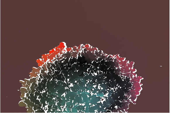
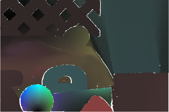
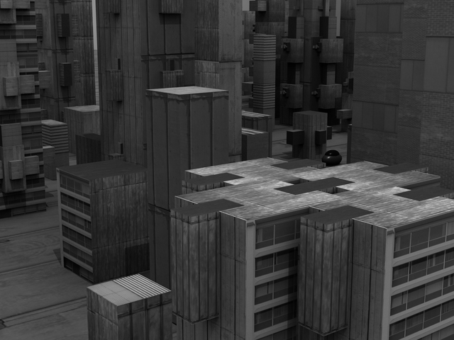
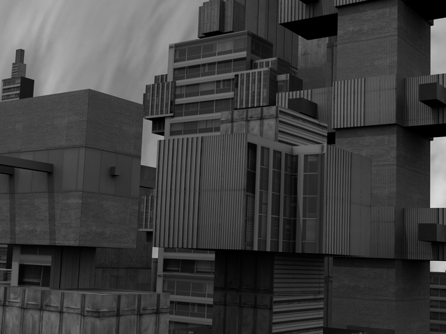
In this section, we show the results of our method for the sequences in the Middlebury benchmark database. We used the method for two different purposes: on the one hand, we seek the best possible results for each sequence; on the other hand, we have also sought a default configuration for the parameters that work appropriately for all sequences.| Frame 10 | Ground truth | Default parameters | Best parameters | |
|---|---|---|---|---|
 |
 |
 |
 |
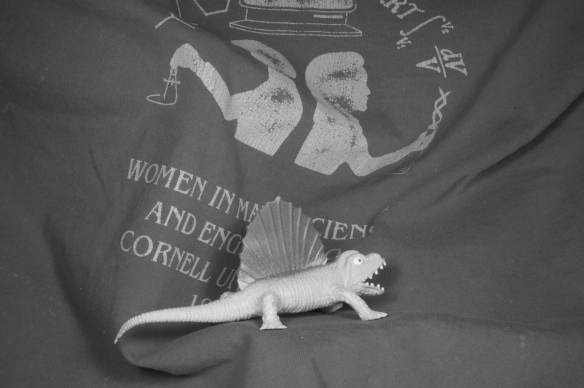
Dimetrodon α=83 γ=48 |
 |
 |
 |
 |
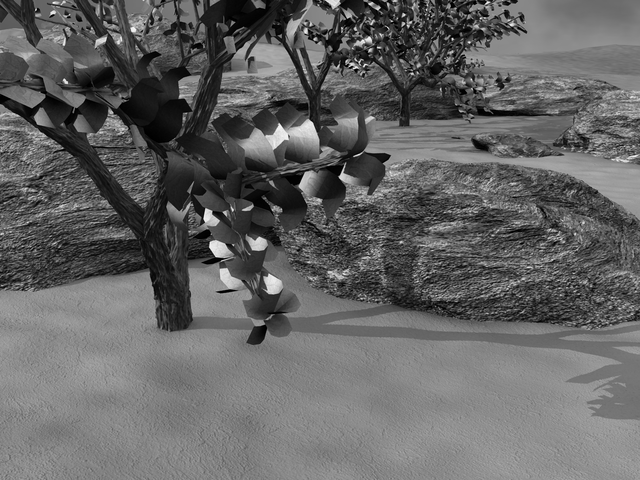
Grove2 α=83 γ=16 |
 |
 |
 |
 |
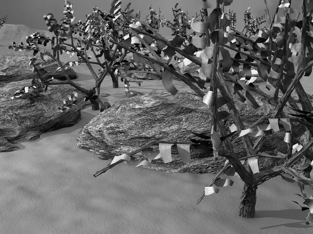
Grove3 α=46 γ=16 |
 |
 |
 |
 |
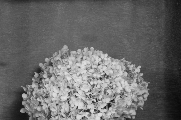
Hydrangea α=104 γ=16 |
 |
 |
 |
 |
RubberWhale α=104 γ=38 |
 |
 |
 |
 |
Urban2 α=51 γ=16 |
 |
 |
 |
 |
Urban3 α=21 γ=16 |
 |
 |
 |
 |
Venus α=21 γ=12 |
| Fig. 3. Several tests with the sequences in the Middlebury benchmark database (Middlebury database) | ||||
| Sequence | α | γ | η | Inner Iter | Outer Iter | EPE | AAE |
|---|---|---|---|---|---|---|---|
| Dimetrodon | 83 | 48 | 0.8 | 30 | 120 | 0.087 | 1.686o |
| Grove2 | 83 | 16 | 0.8 | 25 | 80 | 0.163 | 2.374o |
| Grove3 | 46 | 16 | 0.8 | 29 | 70 | 0.700 | 6.541o |
| Hydrangea | 104 | 16 | 0.8 | 25 | 120 | 0.168 | 2.102o |
| RubberWhale | 104 | 38 | 0.8 | 30 | 120 | 0.111 | 3.751o |
| Urban2 | 51 | 16 | 0.8 | 30 | 120 | 0.340 | 2.667o |
| Urban3 | 21 | 16 | 0.8 | 25 | 100 | 0.492 | 4.234o |
| Venus | 21 | 12 | 0.8 | 27 | 200 | 0.291 | 4.440o |
| Table 2. EPE and AAE for the Middlebury datasets: configuration of the parameters that provide the best average errors. | |||||||
Next, you can see the EPE and the AAE values obtained for the different sequences using as parameters; α=113, γ=83, η=0.8, Inner Iter=25 and Outer Iter=120.
| Sequence | EPE | AAE | |||||
|---|---|---|---|---|---|---|---|
| Dimetrodon | 0.088 | 1.704o | |||||
| Grove2 | 0.227 | 3.027o | |||||
| Grove3 | 0.809 | 7.844o | |||||
| Hydrangea | 0.239 | 2.915o | |||||
| RubberWhale | 0.127 | 4.127o | |||||
| Urban2 | 0.408 | 3.239o | |||||
| Urban3 | 0.512 | 4.392o | |||||
| Venus | 0.300 | 4.580o | |||||
| Table 3. EPE and AAE for the Middlebury datasets: results obtained with default parameters. | |||||||
Acknowledgements
This work has been partially supported by the Spanish Ministry of Science and Innovation through the research project TIN2011-25488.|
|
|