Introduction

We analyse the influence of colour information in optical flow methods. Typically, most of these techniques compute their solutions using grayscale intensities due to its simplicity and faster processing, ignoring the colour features. However, the current processing systems have minimized their computational cost and, on the other hand, it is reasonable to assume that a colour image offers more details from the scene which should facilitate finding better flow fields. The aim of this work is to determine if a multi-channel approach supposes a quite enough improvement to justify its use. In order to address this evaluation, we use a multi-channel implementation of a well-known TV-L¹ method. Furthermore, we review in the original work the state-of-the-art in colour optical flow methods. In the experiments, we study various solutions using grayscale and RGB images from recent evaluation datasets to verify the colour benefits in motion estimation.

Download full text

[1] Monzón López, N, Sánchez Pérez, J& Salgado de la Nuez, A.J.. (2012) Implementation of a Robust Optical Flow Method for Color Images.CTIM Technical Report.(4).Universidad de Las Palmas de Gran Canaria.

Download source code

In this page you can find the code of a multi-channel implementation of a variational technique to determine if the colour information benefits the optical flow calculation. We perform our evaluation with some widely used sequences from the Middlebury benchmark database and the open source movies from the MPI-Sintel flow data set. The code is developed in standard C++ and it has been compiled in Windows and Linux, using the GNU gcc compiler.

multichannel_robust_optic_flow.zip The software is released under the BSD license

You can compile it executing make on the console

Energy model

Let I(x): Ω ⊂ R³ → R be an image sequence, with x=(x,y,t)^T ∈ Ω, I={I^c}_{c=1,...,C} and C the number of channels. We define the optical flow as a dense mapping, w(x)}=(u(x),v(x),1)^T, between every two consecutive images, where u(x) and v(x) are the vector fields that represent the x and y displacements, respectively. We use ∇ I= (I^c_x,I^c_y)^T_{c=1,...,C} to denote the spatial gradient of the image, with I^c_x, I^c_y the first order derivatives in x and y for each information channel. Following the original model, we assume that the brightness constancy assumption is also fulfilled in the multi-channel scheme. Then, according to this notation, our energy functional reads as:

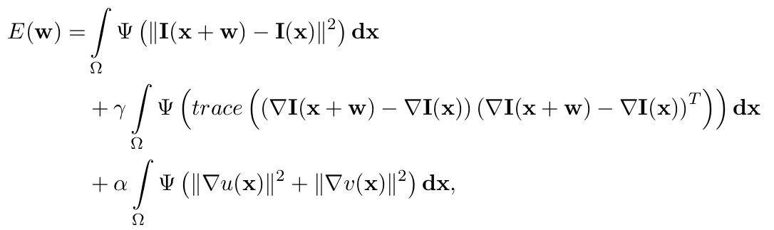
where as a robustification function and ε as a prefixed small constant to ensure that this function is strictly convex. We use the Euclidean norm,

The energy model of Brox et al uses brightness and gradient constancy assumptions in the data term and a TV scheme for smoothing. It depends on the γ and α parameters for controlling the gradient and the smoothness strength, respectively. Notice that the influence of γ is increased proportional to the number of channels. We compensate this situation by adapting the smoothness parameter α, therefore, α = α^′ ∙ C, being α^′ ∙ an input parameter. An example of this multi-channel scheme can be seen in Fig 1.

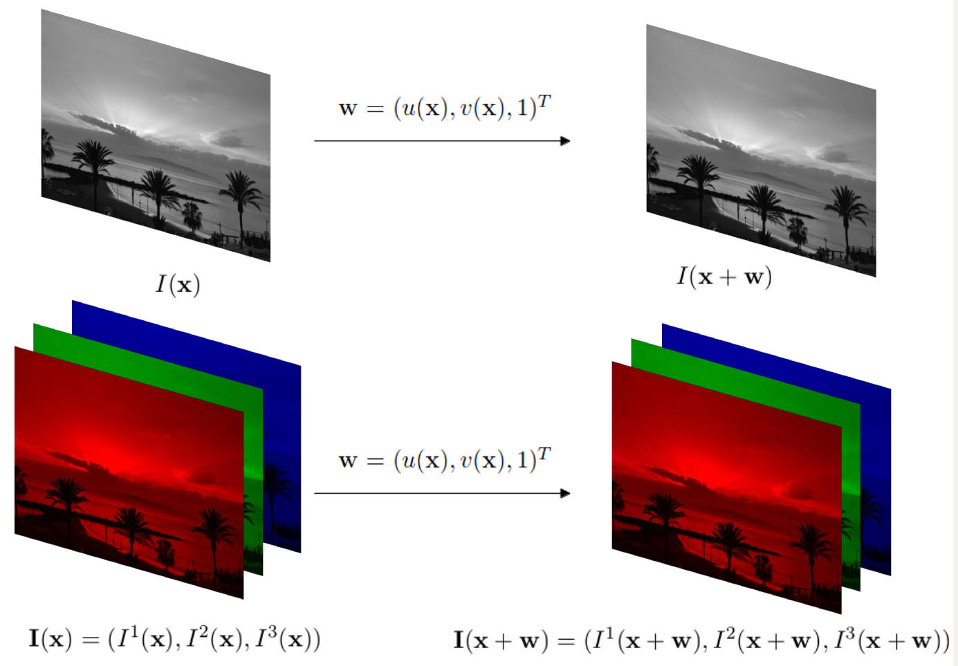
Fig. 1. Notation for grayscale and colour images.

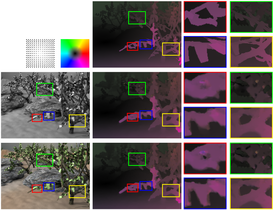
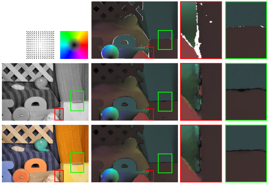
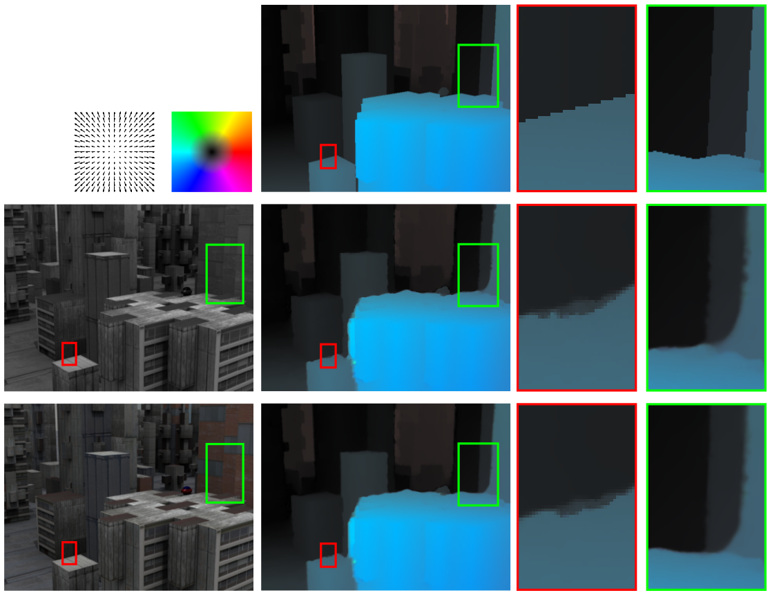
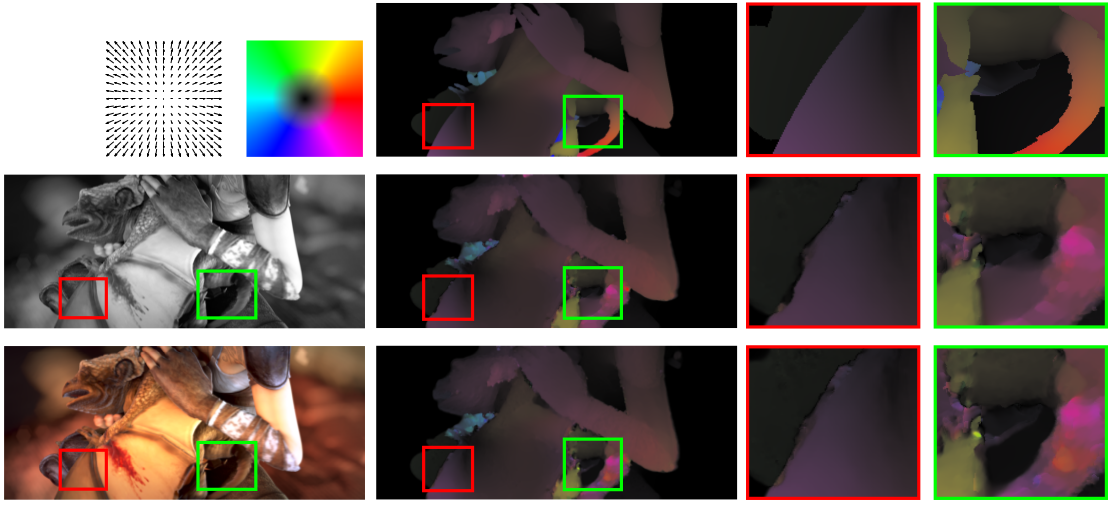
Experimental Results

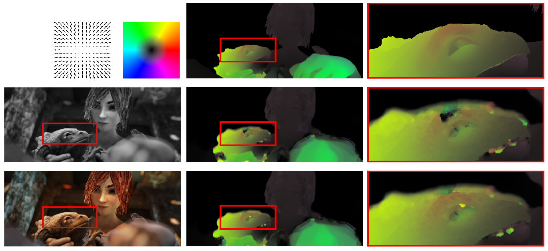
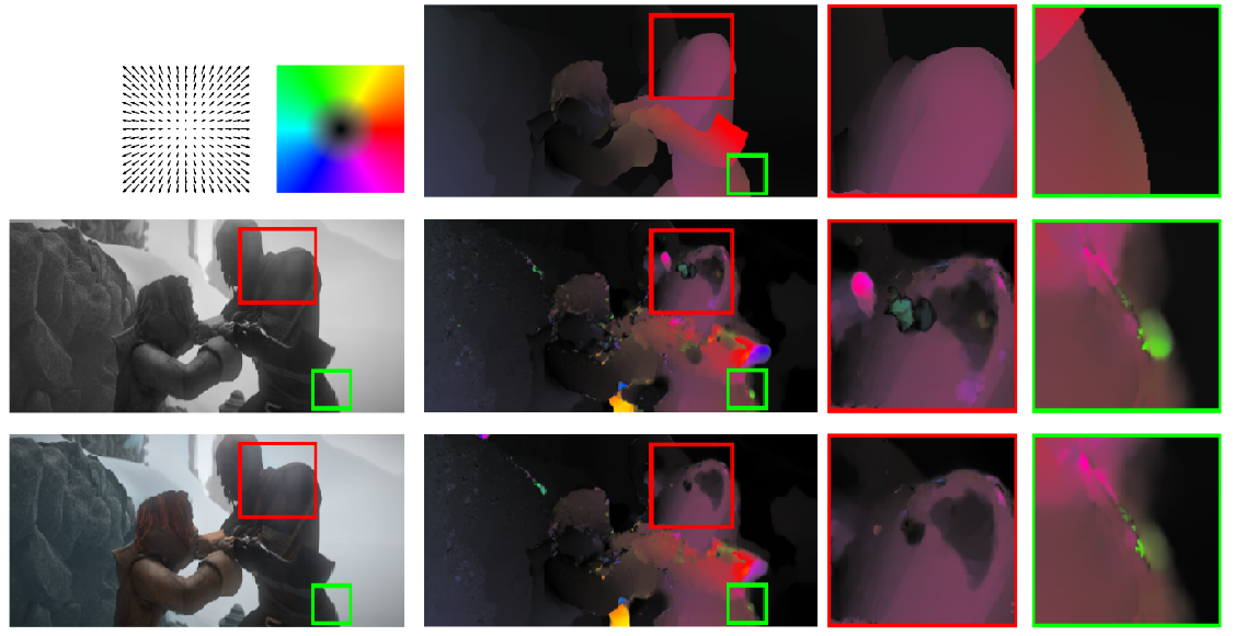
This subsection presents an evaluation of the possible benefits of colour against grayscale information in a variational optical flow method. We show the experiments for some synthetic sequences from the Middlebury benchmark database and MPI-Sintel dataset using RGB and grayscale images. The purpose of these tests is to compare motion details between the best flows achieved for the same sequence.

Figures 2, 3 and 4 show the results for the Middlebury sequences of Grove3, RubberWhale and Urban2, respectively. On the other hand, Figures 5, 6 and 7 depict the best flows and its details for the sequences of Bandage 1, Bandage 2 and Ambush 5 from MPI-Sintel dataset.

In the first column of these figures, we show the colour scheme used for the optical flow representation, the grayscale and the colour images. In the second column, we depict the ground truth and the motion fields for grayscale and RGB, respectively. The remaining columns present motion details for the corresponding solutions. The colour scheme represents the orientation and magnitude of the vector field.

Fig. 2. Motion details for the Grove3 sequence.

Fig. 3. Motion details for the RubberWhale sequence.

Fig. 4. Motion details for the Urban2 sequence.

Fig. 5. Motion details for the Bandage 1 sequence.

Fig. 6. Motion details for the Bandage 2 sequence.

Fig. 7. Motion details for the Ambush 5 sequence.

According to the results, we conclude that the colour information benefits the optical flow estimation. In general, the motion boundaries are better preserved and the error decreases perceptibly, especially in Figures 2 and 7.

Quantitative Results

Next, we show the numerical results provided by the best configurations of α and γ to compare the accuracy of using colour or grayscale in these two datasets. On the other hand, it is interesting to take into account the running times required by the method to justify if the computational cost its reasonable.

First, we depict in Tables 1 and 2 the Average Angular Error (AAE) and the End Point Error (EPE) results for the best settings using the grayscale and colour sequences. The last two columns of these figures show the percentage of error variation between the colour spaces. Observing the results, we can state that the RGB information improves the numerical errors, especially in the Middlebury sequences where most of the amelioration in the EPE exceeds in 5.50% and the AAE in 4%.

Moreover, the enhancement is not so evident in the MPI Sintel sequences. It can be appreciated that, in a few occasions, the colour worsens the EPE. Nevertheless, this deterioration is not excessive and the colour information provides a reasonable improvement in a high percentage of cases, especially in Ambush 5 and Sleeping 1.

The experiments were realized in a computer with the following features: Intel(R) Core(TM) i7 CPU 860 @2.80GHz. We have used a single core in our tests.

	Grayscale		Color (RGB)
Sequence	AAE	EPE	AAE	EPE	AAE(%)	EPE(%)
Grove2	2.198º	0.158	2.169º	0.149	1.34%	2.03%
Grove3	5.971º	0.659	5.661º	0.612	5.48%	7.68%
Hydrangea	2.142º	0.180	2.015º	0.166	6.30%	8.43%
RubberWhale	3.453º	0.103	3.305º	0.097	4.48%	6.18%
Urban2	2.438º	0.359	2.328º	0.340	4.72%	5.59%
Urban3	3.539º	0.386	3.394º	0.401	4.27%	-3.74%
Dimetrodon	1.588º	0.083	1.458º	0.074	8.91%	12.16%
Table 1. AAE and EPE for the Middlebury dataset: configurations of the parameters that provide the best average errors.

	Grayscale		Color (RGB)
Sequence	AAE	EPE	AAE	EPE	AAE(%)	EPE(%)
Alley 1	3.343º	0.374	3.328º	0.373	0.45%	0.27%
Alley 2	3.100º	0.270	3.065º	0.612	5.48%	7.68%
Ambush 2	31.83º	25.14	31.12º	25.22	2.28%	-0.32%
Ambush 4	28.24º	34.73	27.92º	34.72	1.14%	0.03%
Ambush 5	29.59º	2.647	26.91º	2.234	6.80%	18.5%
Ambush 6	12.21º	12.72	11.95º	12.62	2.17%	0.79%
Ambush 7	6.924º	2.072	6.821º	2.152	1.51%	-3.72%
Bamboo 1	4.416º	0.307	4.237º	0.291	4.22%	5.50%
Bamboo 2	6.334º	0.706	6.084º	0.665	4.10%	4.11%
Bandage 1	7.367º	1.061	7.262º	1.030	1.44%	3.01%
Bandage 2	9.403º	1.145	9.242º	1.074	1.74%	6.61%
Cave 2	3.219º	1.707	3.166º	1.741	1.67%	-3.72%
Cave 4	13.19º	7.810	12.60º	7.681	4.68%	1.68%
Market 2	8.814º	1.561	8.628º	1.607	2.15%	-2.86%
Market 5	33.68º	27.37	32.84º	25.08	2.55%	9.13%
Market 6	6.491º	9.245	6.070º	9.036	6.93%	2.31%
Mountain 1	6.500º	1.407	6.296º	1.273	3.24%	10.5%
Shaman 2	6.367º	0.311	6.335º	0.307	0.50%	1.30%
Shaman 3	6.367º	0.508	6.038º	0.520	1.11%	-2.31%
Sleeping 1	1.394º	0.113	1.290º	0.104	8.06%	8.65%
Sleeping 2	1.589º	0.706	1.541º	0.070	3.11%	4.47%
Temple 2	7.579º	1.438	7.296º	1.456	3.88%	-1.24%
Temple 3	3.165º	0.958	2.991º	0.886	5.82%	8.13%
Table 2. AAE and EPE for the MPI Sintel dataset: configurations of the parameters that provide the best average errors.

On the other hand, the error amelioration is not enough to determine if a multi-channel scheme is justified. Thus, Tables 3 and 4 show the runtimes of each sequence and the percentage of improvement provided by the grayscale with respect to the RGB images. As expected, less information means less execution time. However, the difference is not excessively pronounced and, even, in the case of Ambush 2 sequence, less time is required if we use colour information. This means that, using more information from the images, the algorithm usually converges in less iterations. Moreover, we must consider that the increment in the calculations has only affected the data term, so that more image channels does not mean that the operations grow up proportionally.

Sequence	Grayscale	Color (RGB)	Speed (%)
Grove2	45s	67s	32.83%
Grove3	49s	72s	31.94%
Hydrangea	22s	46s	52.17%
RubberWhale	30s	48s	37.50%
Urban2	50s	72s	30.55%
Urban3	55s	81s	32.10%
Dimetrodon	28s	47s	40.42%
Table 3. Computation time in Middlebury sequences.

Sequence	Grayscale	Color (RGB)	Speed (%)
Alley 1	63s	107s	41.12%
Alley 2	49s	81s	39.51%
Ambush 2	199s	150s	-32.67%
Ambush 4	70s	106s	33.96%
Ambush 5	102s	135s	24.45%
Ambush 6	99s	140s	29.29%
Ambush 7	97s	144s	32.64%
Bamboo 1	64s	116s	44.83%
Bamboo 2	79s	108s	26.85%
Bandage 1	89s	128s	30.47%
Bandage 2	93s	128s	27.34%
Cave 2	84s	113s	25.66%
Cave 4	86s	120s	28.33%
Market 2	73s	114s	35.96%
Market 5	205s	205s	0.00%
Market 6	104s	136s	23.53%
Mountain 1	45s	81s	44.45%
Shaman 2	67s	101s	33.66%
Shaman 3	89s	123s	27.64%
Sleeping 1	31s	63s	50.79%
Sleeping 2	36s	68s	47.06%
Temple 2	92s	131s	29.77%
Temple 3	90s	124s	27.42%
Table 4. Computation time in MPI Sintel dataset.